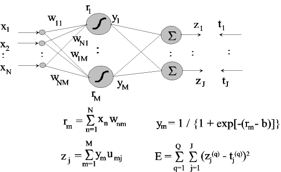
Step 0: read file of feature vector and label
            (target) data {(x^(q), t^(q)): q = 1,...,Q}

Step 1: draw random weights {w_nm: m=1,...,M, j=1,...,J} and
            {u_mj: m=1,...,M, j=1,...,J}
            set step sizes η₁ = 0.5 and η₂ = 0.5,
            set stopping criterion ε = 0.00001

Step 2: for m = 1 to M do
                  compute r_m and y_m

Step 3: for j = 1 to J do
                  compute z_j

Step 4: compute E_new

Step 5: for m = 1 to M do
                  for j = 1 to J do
                        compute u_m,j via steepest descent

Step 6: for n = 1 to N do
                  for m = 1 to M do
                        compute new w_n,m via steeest descent

Step 7: put E_old = E_new
            compute E_new
            if E_new < E_old then
                for k = 1 to 2 do
                        η_k = 1.2η_k
            else for k = 1 to 2 do
                        η_k = 0.9η_k
           increment iteration no. I = I + 1

Step 8: if E_new < ε or iteration I > 1000
                  then stop
            else goto Step 2

Important Notes

(1) The learning rates η₁ and η₂ should be small to start, but with this algorithm they will grow to reach the local minimum rapidly. They will decrease as needed.

(2) An improvement can be made by iterating only on the u_m,j weights for a few iterations and then iterating on the w_n,m weights for a few iterations.

(3) The algorithm should be run several times with different intial weights sets to find a good local minimum where the learning is good.

(4) This algorithm has the disadvantages: (a) there are multiple local minima so the one found may not be global;
(b) the training requires a large number of iterations;
(c) each iteration requires a large volume of computation (although a lot less than the original backpropagation).