The evaluation function for the N cities two dimensional Euclidean TSP is the sum of Euclidean distances between every pair of cities in the tour. That is:
![]()
Where, ![]() ,
, ![]() are the coordinates of city i and
are the coordinates of city i and
![]() ,
, ![]() equals
equals ![]() ,
, ![]() . We also make some changes to the
encoding, selection, and recombination.
. We also make some changes to the
encoding, selection, and recombination.
We need to make some changes to the traditional genetic algorithm to solve TSPs. We do not use binary chromosomes to encode TSPs because TSPs are sequential problems. Instead, we use a path representation where the cities are listed in the order in which they are visited. For example, assuming there are 5 cities 0, 1, 2, 3, 4, if a salesman goes from city 3, through city 0, city 1, city 4, city 2 and returns back to city 3, the chromosome will be 3 0 1 4 2. For an N cities TSP, we initialize the population by randomly placing 0 to N-1 into N length chromosomes and guaranteeing that each city appears exactly once. Thus chromosomes stand for legal tours.

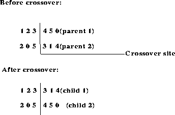
Figure 3: Traditional crossover is not suitable for TSPs
Because of our representation, the traditional crossover and mutation operators are not suitable for TSPs. Figure 3 shows how traditional crossover produces illegal children. The first child is illegal because city 1 and city 3 appear twice, while city 0 and city 5 do not appear at all. The second child is also illegal because city 0 and city 5 appear twice, while city 1 and city 3 do not appear.
There are several crossover operators for TSPs. We use Greedy Crossover which was invented by Grefenstette [Grefenstette 85] in 1985. Greedy crossover selects the first city of one parent, compares the cities leaving that city in both parents, and chooses the closer one to extend the tour. If one city has already appeared in the tour, we choose the other city. If both cities have already appeared, we randomly select a non-selected city.
For example, if we have two parents 1 2 3 4 5 0
4 1 3 2 0 5
To generate a child using the second parent as the template, we select city 4 (the first city of our template) as the first city of the child. 4 x x x x x
Then we find the edges after city 4 in both parents: (4, 5) and (4, 1) and compare the distance of these two edges. If the distance between city 4 and city 1 is shorter, we select city 1 as the next city of child 2. 4 1 x x x x
Then we find the edges after city 1 (1, 2) and (1, 3). If the distance between city 1 and city 2 is shorter, we select city 2 as the next city. 4 1 2 x x x
Then we find the edges after city 2 (2, 3) and (2, 0). If the distance between city 2 and city 0 is shorter, we select city 0. 4 1 2 0 x x
The edges after city 0 are (0, 1) and (0, 5). Since city 1 already appears in child 2, we select city 5 as the next city. 4 1 2 0 5 x
The edges after city 5 are (5, 0) and (5, 4), but city 4 and city 0 both appear in child 2. We select a non-selected city, which is city 3. and thus produce a legal child 4 1 2 0 5 3
We can use the same method to generate the other child. 1 2 0 5 4 3
After crossover, both offspring encode legal tours.
For the same reason that we do not use the traditional crossover operator, we can not use the traditional mutation operator. For example if we have a legal tour before mutation 1 2 3 4 5 0
Assuming the mutation site is 3, we randomly change 3 to 5 and generate a new tour 1 2 5 4 5 0
This new tour is illegal because city 5 appears twice while city 3 does not appear. Instead of using the traditional mutation operator, we randomly select two bits in one chromosome and swap their values. Thus, we still have legal tours after swap mutation as shown in Figure 4.
When using traditional roulette wheel selection, the best individual has the
highest probability of survival but does not necessarily survive. We use CHC
selection to guarantee that the best individual will always survive in the next
generation [Eshelman 91]. In CHC selection if the population size is N, we
generate N children by using roulette wheel selection, then combine the N
parents with the N children, sort these 2N individuals according to their
fitness value and choose the best N individuals to propagate to the next
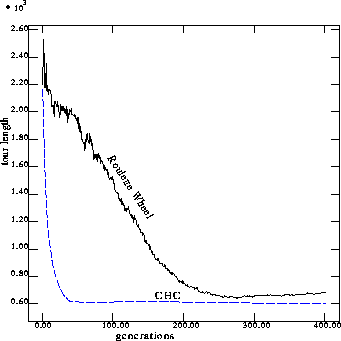
generation. From Figure 5, we can see that with CHC selection
the population converges quickly compared to roulette wheel selection and the
performance is also better. But fast convergence may mean less exploration.
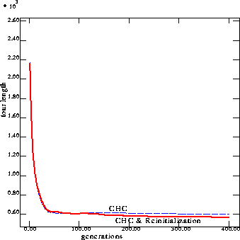
To prevent convergence to a local optimum, when the population has converged we
save the best ![]() of the individuals and re-initialize the rest of the
population randomly. We call this modified CHC selection R-CHC. From
Figure 6, we can see that at first, the performance of CHC and
R-CHC are almost the same, but during later generations the performance with
R-CHC is slightly better than the performance with CHC only.
of the individuals and re-initialize the rest of the
population randomly. We call this modified CHC selection R-CHC. From
Figure 6, we can see that at first, the performance of CHC and
R-CHC are almost the same, but during later generations the performance with
R-CHC is slightly better than the performance with CHC only.

Figure 5: Comparison of Roulette and CHC selection

Figure 6: Comparison of CHC selection with or without re-initialization
We use R-CHC for all the results presented in this paper.