Tuning Genetic Algorithms

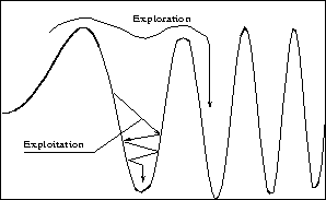
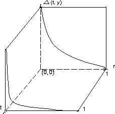
We assume that the polynomial $P(z^{\prime },{\bf q})$ contains nonlinear coefficients, and may therefore have numerous finite local extrema. To enhance the GAs ability to efficiently find a desired global minimum hidden among many local extrema, a good balance between exploration and exploitation is necessary, as shown in Figure 4.

  

Figure 4: Exploration and exploitation

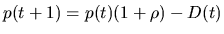
Our strategy is to give GAs a richer population and more exploration to avoid unfavorable local minima in early stages. Later, we gradually reduce the number of such minima qualifying for frequent visits. The attention finally shifts more to smaller refinements in the quality of solution.

Instead of constant population size, we introduce a varying population size schedule by utilizing information about the individual fitness. This has also been investigated in [25,26,27,22].

$$p(t+1) = p(t)( 1+ \rho ) -D(t)$$ (10)

where p(t+1) is the population size for next generation; p(t) is the size of current population; $\rho$ is the reproduction ratio and D(t) is the number of expired individuals. The individual lifetime can be determined by

$$MinLT + \eta\frac{fitness(C^{t}_{i}) - FitMin}{FitMax - FitMin}$$ (11)

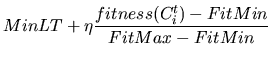
where FitMax and FitMin are maximal and minimal fitness values found until the current generation, respectively. MinLT is minimal allowable lifetime and $\eta$ is a constant which can be set to greater than 1. Although varying the population size introduces additional complexity in out implementation, our tests indicate that the output quality improves significantly and the number of generations needed for searching a desired global optimum decreases compared with the canonical genetic algorithm.

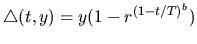
The mutation schedule known as non-uniform mutation can be stated as follows  [27]:

$$\triangle(t, y) = y(1-r^{(1-t/T)^b})$$ (12)

where r is a random number in [0,1], and b is a system parameter determining the degree of nonuniformity, and y equals to (q_k - q_k⁺) or (q_k - q_k^-) for uncertain parameters, (z-1) or (z-0) for the absolute value of the root and $(\theta - \pi)$ or $(\theta - 0)$ for the angle of the root. Figure  5 shows the behavior of mutation operators. The property of this mutation schedule is to help the GA wander freely among local minima at early stages. The attention of mutation then shifts to smaller refinements in the solution at later stages when we are in the vicinity of a possible global optimum. Based on our tests results, a large mutation rate is suggested.

  

Figure 5: The behavior of our mutation operator

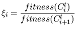
We assume C_i^t and C_i+1^t to be two individuals of population p(t) at generation t. Their offspring for the next generation t+1are generated by linearly combining these two individuals. The resulting offspring are generated by the rules

$$C_i^{t+1} = (1-\alpha\rho_i)C_i^t + \alpha\rho_iC_{i+1}^t$$ (13)

$$C_{i+1}^{t+1} = (1-\alpha\rho_{i+1})C_{i+1}^t + \alpha\rho_{i+1}C_i^t$$ (14)

where $\alpha$ is the value of the random variable distributed on [0,1]. $\rho$ is a bias factor that specifies how much additional information is taken from the dominating individual (higher fitness) in the current stage. The new offspring attempt to inherit the better genes from each of their parent. Assuming maximization problems with a non-negative fitness function, $\rho$ can then be determined from the following equations.

$$\rho_i = \left\{ \begin{array} {r@{\quad: \quad}l} {\xi_i} & if \: \xi_i < 1 \\ { 1} & if \: \xi_i \ge 1 \end{array} \right .$$ (15)

$$\xi_i = \frac{fitness(C_i^t)} {fitness(C_{i+1}^t)}$$ (16)

$$\xi_{i+1} = \frac{fitness(C_{i+1}^t)} {fitness(C_{i}^t)}$$ (17)

Implementing these two equations does not raise the genetic algorithm's computational complexity and, based on our numerical tests, the performance of our modified genetic algorithm is significantly better than that of a canonical genetic algorithm. Figure 6 illustrates this crossover operator. When parent 1 shows better fitness than parent 2, child 1 is allowed to copy additional information from parent 1. As a result, the chromosome of child 1 retains more similarity with parent 1.

  

Figure 6: The mechanism of crossover operator